Tutorial 2: DSP blocks (tiliqua.dsp)
When building audio pipelines, you have the option of re-using cores already present in Tiliqua’s DSP library (connecting them together in different ways), or of building your own DSP blocks from scratch to add to the library.
In this tutorial, we’ll start by implementing our own custom DSP block (a ‘chaos oscillator’, from scratch), and then integrate it with some of the existing blocks. The goal of this tutorial is to add a new DSP block to the library and use it in a new example bitstream in gateware/src/top/dsp, so we can run it on Tiliqua hardware.
Fixed-point Lorenz Attractor
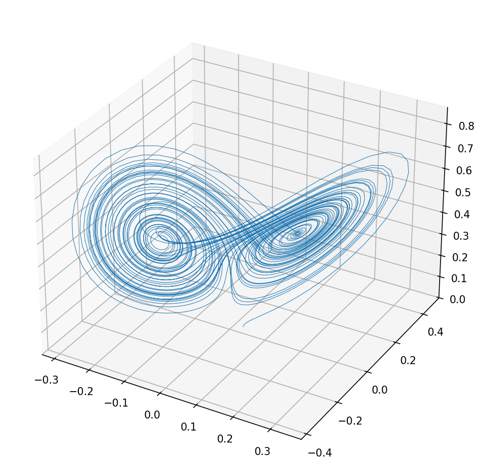
First, let’s construct a new DSP block. We’ll be implementing a Lorenz Attractor. This is a system of equations which, when solved, create an interesting time-evolving 3D pattern like this:
Taking the equations straight from the Wikipedia page:
dx/dt = σ * (y - x)
dy/dt = x * (ρ - z) - y
dz/dt = x * y - β * z

Where the constants:
    σ = 10
    ρ = 28
    β = 8/3
(for the standard Lorenz attractor shape)
Don’t be scared by the derivatives! One way to see the equations as a set of multiplies / adds / accumulations, which when executed iteratively in steps, will create the interesting pattern above.
Oscillator Skeleton
Let’s start by adding a skeleton to the bottom of gateware/src/tiliqua/dsp/oscillators.py:
class Lorenz(wiring.Component):

    # Outgoing sample stream, 3 channels (for X, Y, Z)
    # ASQ is the native sample type (16-bits wide, fixed-point)
    o: Out(stream.Signature(data.ArrayLayout(ASQ, 3)))

    def elaborate(self, platform):

        m = Module()

        # TODO: add logic here

        return m
Note
As we saw previously, a stream.Signature is an Amaranth construct describing a stream of data that is accompanied by a valid/ready handshake. This is a simple protocol used commonly in digital logic. For more details, see Data streams in the Amaranth documentation.
As this is an oscillator with no tuning input, we only have self.o, which is an outgoing stream. The oscillator will be allowed to emit samples as long as the downstream component is ready for one, which is signalled by self.o.ready. As we’ll see, this backpressure will be used to throttle our outgoing samples to exactly match the audio codec sample rate.
Implementing Lorenz
Next, we’ll implement the oscillator logic at the TODO point above. To start, let’s pick a numeric type for our calculations and then define the required constants:
# Type used for internal computations.
# Signed fixed-point, 8 integer bits, 8 fractional bits.
sq = fixed.SQ(8, 8)

# System constants for standard Lorenz shape.
# Cast all floating point values to fit in the fixed-point type above
# (with loss of precision!)
sigma = fixed.Const(10.0, shape=sq)
rho   = fixed.Const(28.0, shape=sq)
beta  = fixed.Const(8.0/3.0, shape=sq)
Note
Note that the sq type has more integer bits than the native audio sample format (which only has 1 integer bit), because the Lorenz calculations span approximately (-30..30), which would overflow 1 integer bit, as we’ll see during simulation.
Note
Be careful when picking fixed-point types, as one ECP5 multiplier takes a maximum width of 18 bits - if your type is larger, more multipliers might be consumed than you expect.
For calculating each iteration and scaling the outputs, we’ll need 2 more constants:
# Timestep - this is how fast our output point X, Y, Z moves around - which is
# directly proportional to the oscillator frequency
dt_inv = fixed.Const(0.01, shape=sq)

# Output scale - Since the equations will emit results between ``(-30..30)`` and
# this component sends native audio samples in the range ``(-1..1)``, we will
# need to scale each point down before sending it out.
scale = fixed.Const(0.015, shape=sq)
Now, we can create 3 registers, one each for the current X, Y and Z position, (as well as their initial values, which are also taken from the Wikipedia page):
# State variables and initial conditions
x = Signal(sq, init=fixed.Const(2.0, shape=sq))
y = Signal(sq, init=fixed.Const(1.0, shape=sq))
z = Signal(sq, init=fixed.Const(1.0, shape=sq))
You will note in the Lorenz equations above, only the current position and some constants appear in them. So, using lib.fixed, we can just write these equations in Amaranth directly:
# Compute derivative terms (without timestep)
dx = sigma * (y - x)
dy = x * (rho - z) - y
dz = x * y - beta * z
This creates 3 new signals, dx, dy and dz, which are combinatorially dependent on x, y and z. That is, they do not change as long as x, y, z do not change.
Finally, we can add the update logic that executes a timestep. This should only happen when the downstream component is ready, so we are only stepping forward in time as fast as the downstream component can consume our outputs:
with m.If(self.o.ready):
    # Update state only when output is consumed.
    m.d.sync += [
        x.eq(x + dx * dt_inv), # x = x + dx/dt
        y.eq(y + dy * dt_inv),
        z.eq(z + dz * dt_inv),
    ]
Now we have a system where x, y and z are evolving, however they are not connected to our self.o output stream. Let’s do that:
# Scale all outputs to fit in [-1, +1]
m.d.comb += [
    self.o.payload[0].eq(x * scale),
    self.o.payload[1].eq(y * scale),
    self.o.payload[2].eq(z * scale),
    self.o.valid.eq(1),
]
Note
In this example, we are also wiring self.o.valid to be permanently asserted. We can do this, because our outputs are always valid. Some components may present invalid outputs or take many clocks to produce the next output, in which case self.o.valid should be deasserted to prevent downstream components from consuming the output sample.
And that’s it! Here’s the complete Lorenz component:
class Lorenz(wiring.Component):

    o: Out(stream.Signature(data.ArrayLayout(ASQ, 3)))

    def elaborate(self, platform):

        m = Module()

        sq = fixed.SQ(8, 8)

        sigma  = fixed.Const(10.0, shape=sq)
        rho    = fixed.Const(28.0, shape=sq)
        beta   = fixed.Const(8.0/3.0, shape=sq)
        dt_inv = fixed.Const(0.01, shape=sq)
        scale  = fixed.Const(0.015, shape=sq)

        x = Signal(sq, init=fixed.Const(2.0, shape=sq))
        y = Signal(sq, init=fixed.Const(1.0, shape=sq))
        z = Signal(sq, init=fixed.Const(1.0, shape=sq))

        dx = sigma * (y - x)
        dy = x * (rho - z) - y
        dz = x * y - beta * z

        with m.If(self.o.ready):
            m.d.sync += [
                x.eq(x + dx * dt_inv),
                y.eq(y + dy * dt_inv),
                z.eq(z + dz * dt_inv),
            ]

        m.d.comb += [
            self.o.payload[0].eq(x * scale),
            self.o.payload[1].eq(y * scale),
            self.o.payload[2].eq(z * scale),
            self.o.valid.eq(1),
        ]

        return m
Testing with amaranth.sim
Amaranth’s built-in simulator provides fantastic infrastructure for testing gateware blocks in Python. Let’s use this to test the Lorenz core we just implemented.
We can start by adding a new test to tests/test_dsp.py:
def test_lorenz(self):

    # Oscillator instance
    dut = dsp.oscillators.Lorenz()

    # Testbench: run it for as long as it takes to compute 5000 samples,
    # and store the samples as arrays of length 3 e.g.
    # points = [[x1,y1,z1], [x2,y2,z2], ...]
    points = []
    async def testbench(ctx):
        for n in range(0, 5000):
            result = await stream.get(ctx, dut.o)
            points.append([r.as_float() for r in result])

    sim = Simulator(dut)
    sim.add_clock(1e-6)
    sim.add_testbench(testbench)
    # Save the waveform dump to a `*.vcd` file viewable in
    # `gtkwave` or `surfer`.
    with sim.write_vcd(vcd_file=open("test_lorenz.vcd", "w")):
        sim.run()
At this point, we probably don’t want to run pdm test to execute every test in the suite, as that can take a while. Instead, to execute only the function we added, we can use something like:
# From `gateware` directory
$ pdm run python3 -m pytest tests/test_dsp.py -k lorenz
Upon opening up test_lorenz.vcd with gtkwave and adding the x, y and z signals to the plot, and then viewing the traces as analog values (again by right-clicking on a signal name in the right panel and setting Data Format->Analog->Step and Data Format->Signed Decimal), you will see:
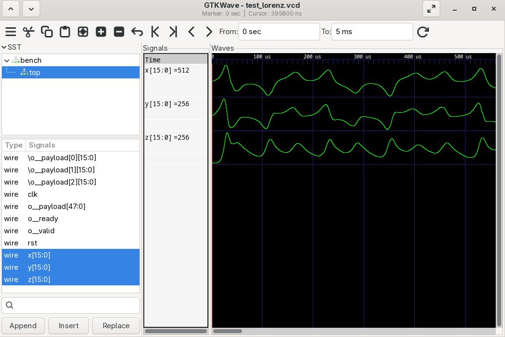
x, y, z starting at their initial conditions and then evolving over time
We could just as easily add the o__payload[n] signals, which are the outputs scaled down to fit in -1..1. Instead, since we collected the output points into points in our test harness above, let’s add some logic to plot them in 3D:
# Append to `test_lorenz`, after `sim.run()` has completed

# Imports here for brevity. Normally you want them at the top of the file
import matplotlib.pyplot as plt
from mpl_toolkits.mplot3d import Axes3D
import numpy as np

# Plot the points in 3D and save to an image.
points = np.array(points)
fig = plt.figure(figsize=(10, 8))
ax = fig.add_subplot(111, projection='3d')
ax.plot(points[:, 0], points[:, 1], points[:, 2], lw=0.5)
plt.savefig('test_lorenz_plot.png', dpi=150, bbox_inches='tight')
Now, on running the test again, we get this nice image saved to test_lorenz_plot.png:
Note
Feel free to experiment with changing the various constants in Lorenz to see if you can make different shapes!
Running on hardware
To run this core on hardware, it first needs to be integrated into a top-level bitstream, which contains all the support logic needed to interface with the outside world. As we saw in the previous tutorial, an easy place to do this is by adding a new core to gateware/src/top/dsp/top.py:
class LorenzAttractor(wiring.Component):

    """
    Lorenz attractor chaotic oscillator.

    Outputs x, y, z on channels 0, 1, 2 respectively.
    """

    # Tiliqua's 'standard interface': 4-in and 4-out audio,
    # as expected by `CoreTop` which contains the required drivers.
    i: In(stream.Signature(data.ArrayLayout(ASQ, 4)))
    o: Out(stream.Signature(data.ArrayLayout(ASQ, 4)))

    # Metadata shown as help in the bootloader
    bitstream_help = BitstreamHelp(
        brief="Lorenz attractor (audio-only!)",
        io_left=['', '', '', '', 'x out', 'y out', 'z out', ''],
        io_right=['', '', '', '', '', '']
    )

    def elaborate(self, platform):

        m = Module()

        # Instantiate our oscillator
        m.submodules.lorenz = lorenz = dsp.oscillators.Lorenz()

        # Split the output channels (1 stream of 3 samples per payload) into
        # 3 independent streams (3 streams each with 1 sample per payload).
        m.submodules.split3 = split3 = dsp.Split(n_channels=3, source=lorenz.o)

        # Merge the 3 independent streams into 1 stream (4 samples per payload),
        # to match the expected output width
        m.submodules.merge4 = merge4 = dsp.Merge(
                n_channels=4, sink=wiring.flipped(self.o))
        wiring.connect(m, split3.o[0], merge4.i[0])
        wiring.connect(m, split3.o[1], merge4.i[1])
        wiring.connect(m, split3.o[2], merge4.i[2])

        # The 4th output channel is unused, we must 'fake' that it is valid
        # so that the stream does not become blocked.
        merge4.wire_valid(m, [3])

        return m
As you can see, there is some stream splitting and merging required here to mate the Lorenz outputs (3 samples wide) with the Tiliqua outputs (4 samples wide). These dsp.Split and dsp.Merge components are commonly used to connect components together that might have different channel layouts. For more information on these, see Stream utilities.
In order to be able to build this core, we’ll need to add a line to the top level CORES array:
# Different DSP cores that can be selected at top-level CLI.
CORES = {
    #                 (touch, class name)
    "mirror":         (False, Mirror),
    "nco":            (False, QuadNCO),
    "svf":            (False, ResonantFilter),
    # ...
    "lorenz":         (False, LorenzAttractor), # <-- add this
}
As a first step, we can run an integration test: that is, our LorenzAttractor core inside CoreTop including simulated drivers and audio codec and so on. This can be done as follows:
$ pdm dsp sim --dsp-core=lorenz --trace-fst
As we saw in the last tutorial, this command emits an *.fst trace of the complete design for debugging, as well as an *.svg that contains a visualization of the output channels. Let’s take a look at the sim-i2s-outputs.svg:
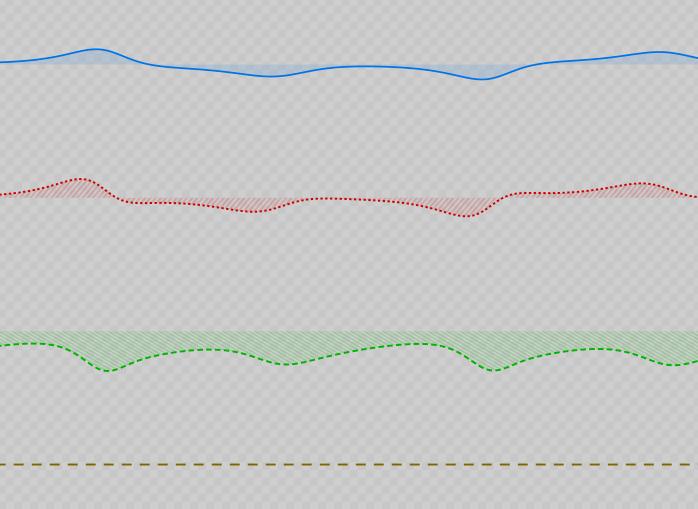
Simulated I2S (codec) outputs of our Lorenz core top-level design
It looks like the audio outputs are evolving as we want. Next, we can build a bitstream for Tiliqua:
$ pdm dsp build --dsp-core=lorenz --verbose
...
Saved to '/home/seb/dev/tiliqua/gateware/build/dsp-lorenz-r5/dsp-lorenz-c3bf5dbf-r5.tar.gz'
Which we can upload to a bitstream slot of our choosing:
$ pdm flash archive --slot 7 build/dsp-lorenz-r5/dsp-lorenz-c3bf5dbf-r5.tar.gz
Because we haven’t integrated any video logic, there will only be audio output. If I connect the outputs over to a second Tiliqua (or an oscilloscope in XY mode), then we get our nice Lorenz attractor shape:
TODO (add nice picture of xbeam visualizing the attractor)
Side quest: squashing multipliers
Looking closely at the synthesis report from our last build build/dsp-lorenz-r5/top.tim, we are consuming loads of multipliers:
Info: Device utilisation:
Info:                 TRELLIS_IO:      66/    197    33%
Info:                       DCCA:       2/     56     3%
Info:                     DP16KD:       0/     56     0%
Info:                 MULT18X18D:      11/     28    39% <-- lots of multipliers!
Info:                     ALU54B:       0/     14     0%
Info:                    EHXPLLL:       1/      2    50%
...
This is to be expected, as we have made no effort to:
Share multiplier tiles amongst the various calculations or
Simplify the calculations to optimize out unnecessary multipliers
Note
One advantage of NOT sharing multipliers is that our Lorenz core can compute new samples at the full system clock rate (i.e. 60MHz). This is because all the multiplies in our logic are happening in parallel, which gives us more speed at the expense of using more FPGA resources, a classic speed-area tradeoff.
For audio applications, it’s usually unnecessary to support such high sample rates, outside of extreme oversampling or low-latency applications.
Let’s try to reduce the amount of multipliers needed by Lorenz.
Multiplies can be shifts
Any time you see a multiplication by a constant, it’s worth asking if that constant could be a power of 2, because this reduces to a simple bit shift. In our set of operations above, we have 10 explicit multiplies:
# ...
dx = sigma * (y - x)                 # 1
dy = x * (rho - z) - y               # 1
dz = x * y - beta * z                # 2
with m.If(self.o.ready):
    m.d.sync += [
        x.eq(x + dx * dt_inv),       # 1
        y.eq(y + dy * dt_inv),       # 1
        z.eq(z + dz * dt_inv),       # 1
    ]
m.d.comb += [
    self.o.payload[0].eq(x * scale), # 1
    self.o.payload[1].eq(y * scale), # 1
    self.o.payload[2].eq(z * scale), # 1
    self.o.valid.eq(1),
]
# ...
Crucially, most of these are multiplies with constants like dt_inv, scale and so on. What happens if we redefine all our constants to the nearest power of 2?
sigma  = fixed.Const(16.0, shape=sq)
rho    = fixed.Const(32.0, shape=sq)
beta   = fixed.Const(2.0, shape=sq)
dt_inv = fixed.Const(1.0/256.0, shape=sq)
scale  = fixed.Const(1.0/64.0, shape=sq)
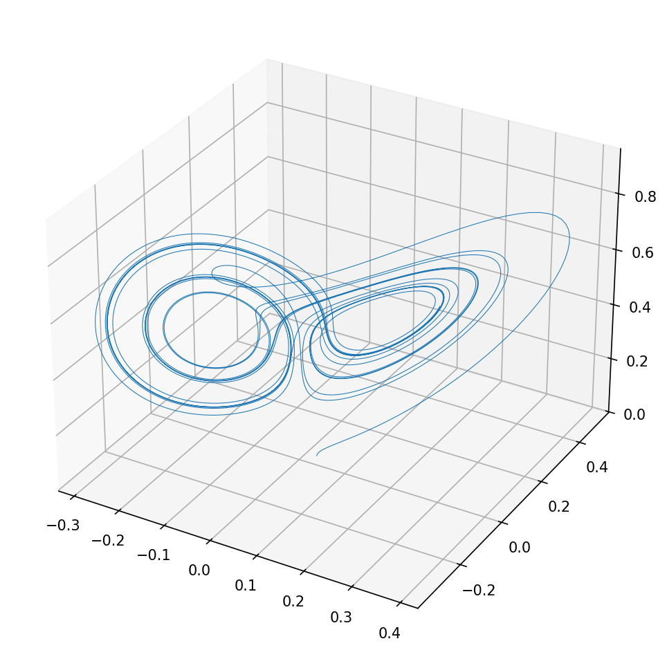
Re-running our test_dsp harness, with this change, we still get a Lorenz-looking plot, albeit with a slightly different shape:
And then on re-synthesis, we now get:
Info: Device utilisation:
Info:                 TRELLIS_IO:      66/    197    33%
Info:                       DCCA:       2/     56     3%
Info:                     DP16KD:       0/     56     0%
Info:                 MULT18X18D:       3/     28    11% <-- less multipliers!
Info:                     ALU54B:       0/     14     0%
Info:                    EHXPLLL:       1/      2    50%
...
By simply rounding constants to powers of 2, we were able to remove 8 multipliers from our design. 1 of these is used by the codec driver for DC calibration, but the remaining 2 are consumed by our core. Can we do even better?
Adding more blocks
Warning
TODO: write this section on adding more DSP blocks to the above example.